Introduction
Mathematical Formulation
The terms ‘nodes’, ‘neurons’, and ‘units’ are used interchangably when referring nodes in the RNN/MLP models. Whereas the biological neurons are only referred to as neurons.
Simplified Network Model
The firing rate of a single neuron is described by the following equation:
\[v_j^t = \gamma \sum_{i=1}^{N} w_{ij} r_i^{t-1} + (1-\gamma) v_j^{t-1}\] \[f_j^t = \left( v_j^t \right)\]- $ r_j^t $: Firing rate of neuron $ j $ at time $ t $.
- $ f(\cdot) $: Activation function.
- $ \gamma $: Decay constant.
- $ w_{ij} $: Weight from neuron $ i $ to neuron $ j $.
- $ v_j^{t-1} $: Membrane potential of neuron $ j $ at time $ t-1 $.
Generalizing to the entire network, we have:
\[\mathbf{v}^t = \gamma \mathbf{W} \mathbf{r}^{t-1} + (1-\gamma) \mathbf{v}^{t-1}\] \[\mathbf{r}^t = f\left( \mathbf{v}^t \right)\]- $ \mathbf{r}^t $: Vector of firing rates for all neurons at time $ t $.
- $ \mathbf{W} $: Weight matrix.
- $ \mathbf{v}^{t-1} $: Vector of membrane potentials for all neurons at time $ t-1 $.
RNN Dynamics
At every timestep, we assume that the neurons in the modeled brain region receive external inputs and signals from their neighboring neurons. These signals are then non-linearly integrated to produce an output. The dynamics of the Recurrent Neural Network (RNN) can be described by the following differential equation:
\[\tau \frac{d \mathbf{v}}{dt} = -\mathbf{v}^t + \mathbf{W}_{hid} f(\mathbf{v}^t) + \mathbf{W}_{in} \mathbf{u}^t + \mathbf{b}_{hid} + \epsilon_t\]- $ \tau $: Time constant.
- $ \mathbf{W}_{hid} $: Weight matrix for the recurrent connections.
- $ \mathbf{W}_{in} $: Weight matrix for the external input.
- $ \mathbf{b}_{hid} $: Bias vector.
- $ \epsilon_t $: Pre-activation noise vector.
Re-write the equation in discrete time, we get an equation looks more similar to the one in the previous section:
\[\Delta \mathbf{v}^t = \frac{dt}{\tau} (-\mathbf{v}^t + \mathbf{W}_{hid} f(\mathbf{v}^t) + \mathbf{W}_{in} \mathbf{u}^t + \mathbf{b}_{hid} + \epsilon_{t}) + \xi_{t}\]- $ \xi_{t} $: Post-activation noise vector.
- $ dt $: Discrete time step (how much time in real world does each time step represent).
Replacing $\frac{dt}{\tau}$ with $\gamma$ gives:
\[\Delta \mathbf{v}^t = \gamma (-\mathbf{v}^t + \mathbf{W}_{hid} f(\mathbf{v}^t) + \mathbf{W}_{in} \mathbf{u}^t + \mathbf{b}_{hid} + \epsilon_{t}) + \xi_{t}\]Model Structure
├── CTRNN
│   ├── RecurrentLayer
│   │   ├── InputLayer (class LinearLayer)
│   │   ├── HiddenLayer
│   ├── Readout_areas (class LinearLayer)
Vanilla CTRNN
A simplistic CTRNN contains three layers, an input layer, a hidden layer, and an readout layer as depicted below.
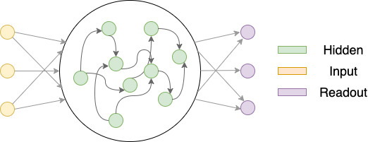
The yellow nodes represent neurons that project input signals to the hidden layer, the green neurons are in the hidden layer, and the purple nodes represent neurons that read out from the hidden layer neurons. Both input and readout neurons are ‘imagined’ to be there. I.e., they only project or receives signals and therefore do not have activations and internal states.
Excitatory-Inhibitory Constrained CTRNN
The implementation of CTRNN also supports Excitatory-Inhibitory constrained continuous-time RNN (EIRNN) similar to what was proposed by H. Francis Song, Guangyu R. Yang, and Xiao-Jing Wang in Training Excitatory-Inhibitory Recurrent Neural Networks for Cognitive Tasks: A Simple and Flexible Framework
A visual illustration of the EIRNN is shown below.
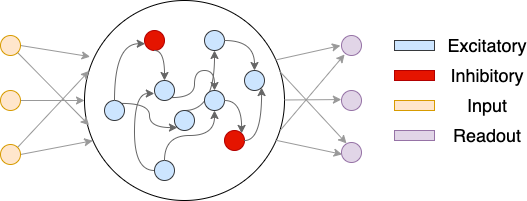
The yellow nodes denote nodes in the input layer. The middle circle denotes the hidden layer. There are blue nodes and red nodes, representing inhibitory neurons and excitatory neurons, respectively. The depicted network has an E/I ratio of 4/1. The purple nodes are ReadoutLayer neurons.